Fix Low Kappa in Screening: Interrater Agreement for Review Teams
Fix Low Kappa in Screening: Interrater Agreement for Review Teams
Cohen’s kappa measures how much two raters agree on categorical judgments after removing the agreement you’d expect from random guessing. It runs from −1 to +1, where 0 means agreement no better than chance and 1 means perfect agreement. Researchers use it most often when two reviewers independently classify the same items, such as screening abstracts as “include” or “exclude” in a systematic review.
TL;DR:
- Cohen’s kappa adjusts raw agreement for chance, so high percent agreement in skewed categories can still result in a low kappa due to high expected agreement.
- When categories are unevenly distributed, kappa can appear misleadingly low even if raters agree on most items, especially in low-prevalence contexts.
- For multiple raters or ordinal data, use Fleiss’ kappa or weighted kappa with quadratic or linear weights, depending on how disagreement severity should be measured.
- In low-prevalence screening tasks, aim for kappa above 0.80 for abstracts and above 0.70 for full texts, and report raw agreement with confidence intervals for full context.
- Automating data extraction and standardization with tools like Papersynapse can reduce disagreement, leading to higher reliable kappa scores in systematic reviews.
Table of Contents
- What Is the Formula Behind Interrater Agreement Kappa?
- Worked Example: Calculating Kappa From a 2×2 Table
- Weighted Kappa and What to Use With More Than Two Raters
- What Counts as a Good Kappa Value?
- Why Does Kappa Sometimes Give Misleading Results?
- How Do You Choose Between Kappa and Its Alternatives?
- How Do You Calculate Kappa in R, Python, or a Calculator?
- How Should You Report Kappa in a Systematic Review?
- How I Think About Kappa Results in Practice
- How PaperSynapse Reduces Extraction Variance in SLR Workflows
- Sources
- FAQ
What Is the Formula Behind Interrater Agreement Kappa?
Kappa compares what your raters actually agreed on against what they’d agree on by pure luck. The formula is deceptively short: κ = (po − pe) / (1 − pe). Every argument about kappa’s quirks traces back to what those two terms mean and how they’re built.
Po is the observed proportion of agreement. Add up the items where both raters gave the same label, divide by the total number of items, and you have po. If two reviewers screened 100 abstracts and agreed on 85 of them, po = 0.85. That part rarely confuses anyone.
Pe is where people get tripped up. It’s the agreement you’d expect if both raters were labeling items randomly, but weighted by how often each rater actually used each category. You calculate it from the marginal proportions, the row and column totals in your contingency table, not from a flat 50/50 assumption. For a binary “include/exclude” decision, pe equals the probability both raters say “include” by chance plus the probability both say “exclude” by chance. If Rater A includes 40% of abstracts and Rater B includes 50%, the chance-both-include term is 0.40 × 0.50 = 0.20. Do the same for “exclude,” add the two products together, and that sum is pe.
The subtraction in the numerator, po − pe, tells you how much agreement survives once you strip out the luck component. Dividing by (1 − pe) rescales that surviving agreement against the maximum possible improvement over chance. It’s a normalization step, not decoration.
One edge case trips up people running this by hand: when pe approaches 1, the denominator shrinks toward zero and kappa becomes unstable, swinging wildly for tiny changes in po. This happens when raters use one category almost exclusively, which is common in low-prevalence screening tasks where most items get rejected. A kappa calculated on a 98/2 split deserves a second look before you trust it at face value, a point that resurfaces later when the prevalence paradox comes up.
Cohen introduced this correction-for-chance approach in the 1960s specifically because raw percent agreement inflates apparent reliability whenever categories are unevenly distributed. Two raters who both classify 95% of items as “normal” will show 90%+ raw agreement even if they’re barely paying attention. Kappa exists to catch that.
Worked Example: Calculating Kappa From a 2×2 Table
Numbers make this concrete faster than any explanation. Say two reviewers screened 100 titles for a systematic review, deciding “include” or “exclude” for each one.
| Rater B: Include | Rater B: Exclude | Row Total | |
|---|---|---|---|
| Rater A: Include | 40 | 10 | 50 |
| Rater A: Exclude | 5 | 45 | 50 |
| Column Total | 45 | 55 | 100 |
Here’s the calculation, step by step:
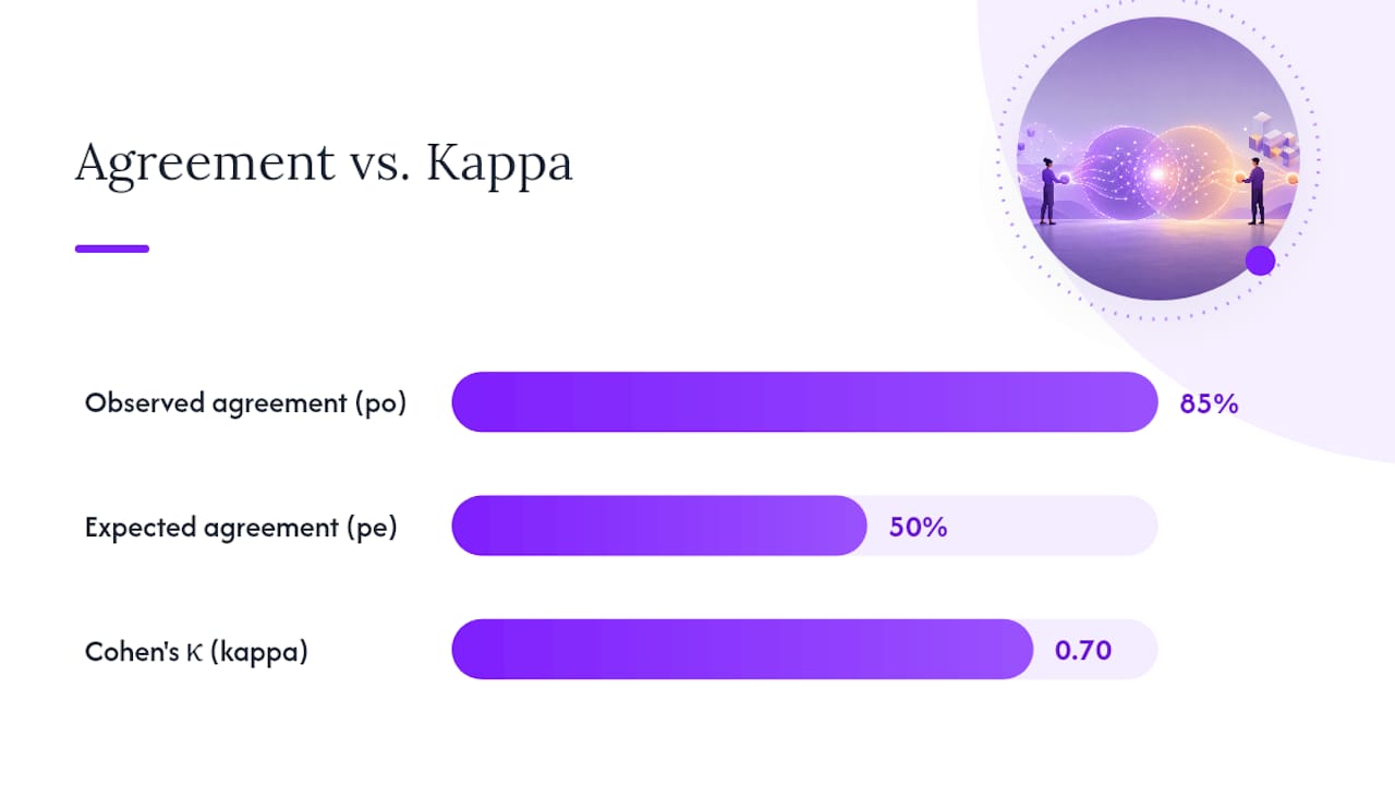
- Find po. The raters agreed on 40 “include” decisions and 45 “exclude” decisions, for 85 agreements out of 100 items. Po = 85/100 = 0.85.
- Find the marginal proportions. Rater A included 50% of items and excluded 50%. Rater B included 45% and excluded 55%.
- Calculate pe for “include.” Multiply the two marginal proportions for that category: 0.50 × 0.45 = 0.225.
- Calculate pe for “exclude.” Multiply the marginals for that category: 0.50 × 0.55 = 0.275.
- Sum both terms. Pe = 0.225 + 0.275 = 0.50.
- Apply the formula. κ = (0.85 − 0.50) / (1 − 0.50) = 0.35 / 0.50 = 0.70.
A kappa of 0.70 lands in the “substantial” range on the interpretation scale covered later, but notice something important: raw agreement was 85%, which sounds excellent on its own. Kappa knocks that down to 0.70 once chance is removed, a 15-point drop that raw percentages alone would never reveal.
Two arithmetic mistakes show up constantly in manual calculations. First, people compute pe using a flat 0.5 chance rate instead of the actual marginals, which only works when both raters split their decisions exactly 50/50. Second, people forget that po and pe both need to be proportions, not raw counts, before you subtract and divide.
For reporting, always pair your point estimate with a confidence interval. A kappa of 0.70 calculated on 20 items carries far less certainty than the same value calculated on 500 items, and most statistical software (covered in the tools section below) will output the CI alongside the point estimate without extra work on your part.
Weighted Kappa and What to Use With More Than Two Raters
Unweighted kappa treats every disagreement as equally bad, which works fine for nominal categories like “include” versus “exclude” but falls apart for ordinal data. If two raters rating study quality on a 1 to 5 scale disagree by one point (a 3 versus a 4), that’s a minor slip. If they disagree by four points (a 1 versus a 5), that’s a real problem. Standard kappa can’t tell the difference. Weighted kappa fixes this by assigning partial credit based on how far apart the two ratings fall.
- Linear weights penalize disagreements in direct proportion to the distance between categories. A two-point gap costs twice as much as a one-point gap.
- Quadratic weights penalize larger gaps disproportionately harder. A two-point gap costs four times as much as a one-point gap, because the penalty is squared.
- Use linear weighting when you consider all size-of-error differences roughly equally serious in real-world consequence.
- Use quadratic weighting (the more common default in practice) when large disagreements represent a qualitatively different kind of failure, not just a bigger version of a small one.
Weighted kappa still assumes exactly two raters and ordinal or interval-like categories. Once your design changes, you need a different tool entirely.
Fleiss’ kappa extends the same chance-corrected logic to three or more raters evaluating the same set of items, which is the standard choice for systematic review teams running three-reviewer screening panels. Krippendorff’s alpha handles an even wider range of situations: missing data, unequal numbers of raters per item, and multiple levels of measurement (nominal, ordinal, interval, ratio) within one coherent framework, which makes it the more flexible option for messy real-world coding projects. The intraclass correlation coefficient (ICC) applies when the ratings themselves are continuous, like measuring a tumor diameter in millimeters rather than sorting it into a category. Each of these exists because Cohen’s kappa’s assumptions about two raters and categorical data are restrictive by design, not because kappa is flawed.
What Counts as a Good Kappa Value?
Landis and Koch’s 1977 benchmarks remain the most widely cited interpretation scale in the field, and nearly every methods section that reports kappa references them in some form.
- 0.00 to 0.20: slight agreement
- 0.21 to 0.40: fair agreement
- 0.41 to 0.60: moderate agreement
- 0.61 to 0.80: substantial agreement
- 0.81 to 1.00: almost perfect agreement
Treat these bands as a shared vocabulary, not a scientific law. The original PMC review on the kappa statistic notes that Landis and Koch essentially proposed these cutoffs by convention, and several methodologists argue they’re too forgiving for high-stakes clinical or diagnostic research, where a kappa in the “moderate” range might still represent an unacceptable error rate.
In systematic review screening, teams commonly report abstract-screening kappas around 0.82 and full-text screening kappas around 0.77, according to a mixed-methods review of literature-review reliability. That gap between stages isn’t noise. Full-text decisions are usually harder calls than abstract triage, and the numbers reflect that.
Rather than anchoring only to Landis and Koch, set pragmatic thresholds by task. For abstract screening, aim for kappa above 0.80 before trusting a single reviewer to work independently on the remainder of the corpus. For full-text screening, 0.70 to 0.75 is a defensible working baseline given how much more judgment full-text decisions require. For data extraction on structured fields, push for 0.85 or higher, since extraction errors propagate directly into your review’s results. Whatever threshold you land on, report the raw percent agreement and a confidence interval next to the kappa value. A bare number with no context tells the reader almost nothing about how confident to be.
Why Does Kappa Sometimes Give Misleading Results?
Kappa’s most counterintuitive behavior is the prevalence paradox: when almost all items fall into one category, kappa can look surprisingly low even when raters agree on nearly everything. Picture two reviewers screening 500 abstracts where 480 are obvious excludes and only 20 are genuine candidates for inclusion. If the raters agree on 470 of the excludes and split evenly on the 20 marginal cases, raw agreement sits above 95%, but kappa can drop into the “moderate” range or lower because pe is already high when one category dominates the marginals. The tutorial on computing interrater reliability walks through exactly this dynamic, and it’s the single most common source of “why is my kappa so low when we agreed on almost everything” confusion in screening projects.

Bias works differently but causes similar confusion. If one rater systematically includes more items than the other, even while their underlying judgment is similar, the asymmetry in their marginal totals changes pe and can push kappa in either direction depending on the specific pattern. Two raters with identical accuracy but different thresholds for “borderline include” will show a different kappa than two raters who share the exact same threshold, even if both pairs are equally skilled.
Pro Tip: When kappa looks lower than your gut says it should, decompose disagreement into its “quantity” and “allocation” components before assuming your raters are unreliable. Sometimes the raters agree closely on how many items belong in each category, they just disagree on which specific items, and that distinction changes what you do next.
Three mitigations handle most cases:
- Report percent agreement alongside kappa every time, since the gap between the two numbers is itself diagnostic information.
- When category prevalence is extreme, supplement kappa with Cramér’s V or a direct quantity/allocation breakdown to keep the interpretation transparent.
- Treat a surprisingly low kappa as a prompt to re-examine your codebook, not as proof your raters can’t be trusted.
How Do You Choose Between Kappa and Its Alternatives?
Picking the right reliability statistic comes down to three questions: how many raters, what kind of data, and how skewed are your categories.
- Two raters, nominal categories with no natural order (include/exclude, present/absent): use standard Cohen’s kappa.
- Two raters, ordinal categories with a meaningful order (quality ratings on a 1 to 5 scale): use weighted kappa, choosing quadratic weights if larger gaps should be penalized more heavily.
- More than two raters, categorical data: use Fleiss’ kappa for a straightforward multi-rater extension, or Krippendorff’s alpha if you have missing ratings or mixed measurement levels.
- Continuous measurements (blood pressure readings, tumor size, duration in minutes): use the ICC rather than any kappa variant.
- Rare-category situations, where one label dominates 90% or more of your data: always report raw percent agreement next to whichever statistic you choose, and consider a secondary index like Cramér’s V for triangulation.
None of these rules require memorizing a decision tree. They follow directly from what each statistic was built to handle. Kappa variants exist for categorical judgments made by a bounded number of raters. ICC exists for measurements on a continuous scale. Once you know your data type and rater count, the choice mostly makes itself.
How Do You Calculate Kappa in R, Python, or a Calculator?
You rarely need to compute kappa by hand past the first time you learn the formula. Every major statistical environment has a built-in function, and cross-checking two tools against each other is good practice before you commit a number to a manuscript.
- In R, the
irrpackage’skappa2()function takes a two-column data frame of ratings and returns kappa directly. Thepsychpackage’scohen.kappa()function goes further, returning both unweighted and weighted kappa along with confidence intervals in a single call, which saves you from computing CIs by hand. - In Python,
sklearn.metrics.cohen_kappa_score()takes two arrays of labels and returns the kappa statistic in one line. It doesn’t compute a confidence interval natively, so you’ll need to bootstrap one yourself or pair it with a separate statistics library if a CI is required for publication. - Spreadsheet users can build the formula directly from a contingency table using SUM and basic arithmetic, following the same six steps shown in the worked example above. This is worth doing at least once, purely so the formula stops feeling like a black box.
- Online calculators exist for quick sanity checks on small tables, though for anything going into a published manuscript, run the numbers through R or Python so you have a reproducible script alongside the result.
Pro Tip: Never trust a single tool’s output blindly, especially on your first calculation with a new dataset. Run the same contingency table through two different implementations, one in R and one in Python, and confirm they agree to at least three decimal places before reporting the number anywhere.
How Should You Report Kappa in a Systematic Review?
Aggregating one overall kappa across your entire systematic review process hides more than it reveals. Abstract screening, full-text screening, and data extraction are different tasks with different error patterns, and lumping them into a single number obscures exactly where your review’s weak points sit. Stage-specific reporting is the standard recommendation, and it’s supported by research into interrater reliability in review methodology showing that coder decision-making varies meaningfully across stages.
- Report a separate kappa (with confidence interval) for abstract screening, full-text screening, and data extraction rather than one blended figure.
- Pair each kappa with the raw percent agreement for that stage, since the gap between the two numbers flags prevalence effects.
- Document your training and pilot process: how many items the pilot round covered, how disagreements were resolved, and whether the codebook changed as a result.
- Specify your conflict-resolution method, whether that’s a third reviewer, discussion to consensus, or a predefined tie-breaking rule.
| Reporting element | What to include |
|---|---|
| Contingency table | Full counts for each rater pair at each stage |
| Kappa with CI | Point estimate plus confidence interval, not kappa alone |
| Percent agreement | Raw agreement reported alongside kappa, every stage |
| Training and piloting | Pilot round size, codebook revisions, calibration steps |
| Resolution process | How disagreements were adjudicated |
Realistic baselines help set expectations before you start. A review found stage-specific averages indicating strong agreement for abstract screening and data extraction, and slightly lower agreement for full-text screening. If your team’s numbers fall well below those figures on a first pilot round, that’s a signal to revise the codebook or run another calibration exercise before scaling up to the full corpus.
How I Think About Kappa Results in Practice
A low kappa is information, not a verdict on your team’s competence. It usually points to an ambiguous codebook, an undertrained rater, or a genuinely hard category boundary, and each of those has a different fix. Piloting on a small batch before full-scale screening, then holding a consensus meeting to argue through the disagreements, raises kappa more reliably than simply retraining people to “try harder.”
The same logic applies once AI enters your extraction workflow: set an expected human-AI agreement baseline before you rely on automated output, and verify it the same way you’d verify a second human coder, not with blind trust.
— Ubada
How PaperSynapse Reduces Extraction Variance in SLR Workflows
Manual extraction is where most interrater disagreement actually happens, not in the screening decisions researchers usually calibrate for. Papersynapse gives systematic reviewers one integrated workflow instead of the usual patchwork: import references from Scopus or Web of Science, extract data with AI directly from abstracts, normalize labels across your dataset, and visualize results, all inside a single platform rather than stitched together across spreadsheets and separate tools.

That matters for interrater agreement kappa specifically because most extraction variance comes from two coders reading the same abstract and applying a category label slightly differently, the exact ambiguity a shared, structured extraction schema is built to close. When every reviewer’s output runs through the same fields and the same normalization step, you remove a whole category of disagreement before it ever shows up in your contingency table. Teams running protocol-driven extraction get a head start on the consistency that a strong kappa depends on.
Papersynapse offers tiered subscription plans scaled to how many papers you process. If extraction consistency across your review team is a recurring headache, start with the free tier on the Papersynapse platform and run your next batch of abstracts through it before your team’s next calibration round.
FAQ
What Is Interrater Agreement?
Interrater agreement measures how consistently two or more independent raters classify the same items using the same categories or scale. Cohen’s kappa is the most common statistic for quantifying it when two raters use categorical labels.
How Do You Interpret a Kappa Agreement Score?
Using the Landis and Koch scale, a kappa between 0.61 and 0.80 indicates substantial agreement, and 0.81 to 1.00 indicates almost perfect agreement, though these cutoffs are widely treated as conventions rather than fixed rules. Always interpret the number alongside percent agreement and a confidence interval rather than in isolation.
What Is Considered a Good Kappa Statistic?
For systematic review screening, a kappa above 0.80 for abstract screening and above 0.70 for full-text screening are reasonable working baselines, based on typical values reported in the review literature. For data extraction tasks, aim higher, since extraction errors carry directly into your results.
Can You Use Cohen’s Kappa for Three Raters?
No. Cohen’s kappa is defined for exactly two raters; with three or more, use Fleiss’ kappa or Krippendorff’s alpha instead, both of which extend the same chance-corrected logic to multi-rater designs.
Does Papersynapse Calculate Kappa Automatically?
Papersynapse focuses on standardizing and automating the extraction step itself, reducing the raw disagreement that shows up when reviewers code data by hand. Current plan details and pricing are available on the Papersynapse site.